Dr. McWillie

Bitcoin is literally a toy people use for fun activities such as executing contracts (“blow up this bridge / solve this math problem and I will give you $5 / a Delta Force Fentinyl Lollipop) … and nothing else.

This entire media landscape is as absurd as saying “The Chess Industry was Ruined by Magnus.” Or “Playing Chess will Destroy All the Trees to Make the Boards!”

There are still maybe 12-14 people alive, on earth, not in jail, who can explain what *is* a bitcoin, or have *seen* The Actual Blockchain.

Are you one of them? No.

Do you know one of them? Doubt it.

Do you think someone will tell you? Good luck / get plucked.



The driver of waste and regulatory capture keeps creeping back in because people want to make money off of adding an abstraction layer to something that was designed specifically not to have any abstraction layers. We saw this repeatedly in business school, where people would deadass with a straight face say “we can get businesses to use it as a perk” and take $500 from each employee to give them a $10 voucher that has no value in the future. In biology, we call that churn: Parasitic.

Meaning: China is absolutely correct for saying it’s a waste, and the US is absolutely correct in just storing raw BTC instead of letting private sector repeatedly thrash the economy demanding a market suddenly be created for wares no one needs. Because it’s a waste: BTC is in a sense, the bottles and cans left over from a party.

You can re-use them for whatever you want but they are still toxic waste barrels no matter what gets slapped on them. That’s where I see the wastage and overhead come in. Instead of making warehouses and terminals, people have made arbitrage and speculation platforms, anticipating that these are goods and not … cargo containers.

What *is* of value? The entire Blockchain. The Satoshi sector.

How do you get value out of those? By not diluting them with service layers that cost money to make and therefore have to recover on investment. No one claims we need to make the trains, roads, and landfills pay for themselves — so I think again, and why Satoshi thinks all of you suck, is that you keep trying to steal Lego from people having fun, and spray-glue it into a product, box it, ship it around the world, sell it, and keep it in an expensive storage place. Eventually that bill has to be paid, but this bundling is non-essential / rent-seeking.

The Mars Helicopter Company has a unique role in the current tech environment. The Company formed to bring the NASA Ingenuity Helicopter to Mars and keep it running: https://www.nasa.gov/news-release/after-three-years-on-mars-nasas-ingenuity-helicopter-mission-ends/

We have four complimentary goals:

1) Medical and Philanthropy: We are actively deployed to every continent, including Antarctica, providing medical and veternarian services to stranded, isolated, threatened, and impoverished populations.

2) Artificial Intelligence and Machine Learning: Your competition is trying to convince you their “three LLMs in a trenchcoat” is something it isn’t. We have access to entire planets of compute, cooled in outerspace. And you wish you could access our agents.

3) Aviation: Our core mission is aviation development, from pilot training to safety devices

4) Mineral Extraction: Yep. We drill, baby. Mars is just our staging area. We have an entire galaxy to explore!

Captain Scumbeard and the Whorehouse Tri-lemma, an Ancient Levantine Sailor’s Tale
(Yes, this is an actual Pythagorean text, it was suppressed by Saddam Hussein)

In response to: https://blog.computationalcomplexity.org/2024/08/determing-which-math-problems-are-hard.html

In Ancient Greece, Muff and Man Problems where when the Pirate Captain saw a Trojan Whore House and then said AYYYY HOW MANY BAWSACKS WE FINNA DRAIN
and the seamen had NO idea what the captain said because half his teeth were rotten away from drinking self-brew wine

so they crashed into the brothel with the boat because the boat is just a large horse cock that can float… and had to save all the whores from the whitewater rapids, so every sailor’s room had to also have at least one hooker in it (a Tzaddi as they say in Aramaic) in case the prostitutes fell overboard

so, given that every prostitute has a giant hairy cynthia, how many seamen will need to unclog the toilets every hour, if there are 12 shitters, 37 sisters, 91 seamen, and a grapey pirate captain?

and if there is an overflow, demonstrate using tri-modal logic, which side will capsize?

Dear NASA Damage Control
CC: Laurie Leshin,

I don’t know what Girl Scouts of the USA badge I earned for this one. But it was never about a badge. It was about making sure no one gets in an accident on a helicopter. Why me though?

Why not ask the AI? Or the Air Force? Why someone in the Army? Well, my relationship to aircraft is “get out of them as soon as possible and carry the pilot(s) and the bud/s home with you.”

That’s it. I don’t have the laser beams or the doomsday cannon. I’m just, along for the ride and have bandaids and a barf bag.

So someone asked — what flight experience do you have?
Well. A long time ago, I knew someone really inspiring. And becoming a pilot meant a lot to him. For some reason, our command convinced him I was going to take his flight school slot. But if they offered me that school, I would say — the choice is not up to me.

So we got what we both wanted.

My flights include: SV-22, Ka-52M, YSH-2G, SH-2G.
And that’s it. I’m no one special. The vehicles are. The other pilots are.

Why those? Because those are the ones that are used for the important people. But they are also dangerous to fly. So I wanted to make sure I understood how these work before someone I cared about stepped into them and took to the skies.

Still, people get the wrong idea because small things on Mars can cast huge shadows. I worked on the Mars Helicopter, not because I was “good” at this (see above — I was last pick for flight school). It was because I wanted to make sure that as the pandemic happened, my colleagues didn’t lose their job. They hired me to write the “control mechanism” that shuts down the helicopter and then the 200+ engineers and 20000+ contractors go home, and have nothing to do, because there would have never been another project like that for awhile, and the private Mars helicopter industry is still very small.

So I just took home a NASA Jet Propulsion Laboratory laptop, and fixed the descent and landing and simulation code instead. For safety. But also, another secret thing: to keep people from starving.

That is why it was named the Artemis project — a long time ago, a group of people who were all unified by just… not being as smart as Athena nor as tough as Zeus nor as beautiful as Aphrodite and certainly not as rich as Hades … found themselves stuck in a dusty office with burnt out electronics and Dell Xeon Workstations that Voted for Bill Clinton… and just got to work with their bolts and arrows in the forests of La Cañada-Flintridge in case the rest of the village’s voyage at sea netted no fish.

We did this because we volunteered. We didn’t see it as “getting fired” — we saw this as buying time.

Every rotation of each rotor on Mars, taught everyone on Earth something about helicopters and how the atmosphere affects their reliability. Why did we do this on Mars?

So some day, somewhere, even some bad guy’s life might be saved. It’s just that important.

Sincerely,
That One Astronaut who missed the Bus but didn’t get the memo
PS: Where are you? Mars isn’t that bad!

And then I finished school and was immediately told my skillset was out of date. So I remembered what was important to me all along: Seeing the stars.

Where did all of this start? What changed me into a MAD scientist?

Anyways when I was taking Calculus II for the 20th vain attempt, but this time for real, my ancestral homeland fell under an unprovoked attack on the 100 year anniversary of our genocide. My tutor had to flee and I had to suddenly meet “my people” along with a rag-tag legion of mercenaries and furloughed IT workers and corporate consultants who saw no future in “The Same Thing Forever.”

In my own personal story, my wonderful NIST internship contract was revoked between year two and three, and then I just fell through the cracks. Maybe NASA forgot to look at my space cadette application. The US Army forgot I signed an indef contract. You find yourself in the same place but the world changes. Reality and digitality converge and every human interact suddenly became reduced to a stack of contracts that had to ezero out against another stack of contracts.

Every tear told a story, and I made so many friends along the way.

I guess I’ll never find out the secret of Calculus III — where they get to switch from cow culos to Chaos Culos.

I think at the end of the day, the one thing I wanted before I even became a Girl Scout, before I tried to earn my Green Beret, before I even went to NASA thinking I would ever make it: the one thing I alwayever wanted was to take my telescope really far away from everyone and look at the stars. Whenever I would do this, these weirdos would show up trying to smash all my stuff saying it was dangerous. The people who attacked that village when I was taking Calculus II, for example, are the telescope smashers.

I decided to create a chemical weapons company that focuses specifically on bionic acrylic nails that can get through metal detectors and make people type really quickly on all these devices that are meant to artificially frustrate us only to lease us back the ability to use them with less frustrations.

I have always been a lover, not a fighter, and what I realised is that women’s nail products slow them down and most of that is made for this generic “average finger shape” that no one actually has. I have seen everyone’s hands across the world. Some people have different nail shapes than others, but keyboards were largely a US-UK-EU innovation. There are some people who tell me they literally can’t type because they have to curl their fingers inward / obliquely, especially because low-flight laptop keyboards became the norm. It’s weird. Maybe that’s what holds people back. Maybe these keyboards keep getting shittier and smaller as a push towards just getting rid of humans from the equation, or ultra-optimising these to be toys or labour-generating devices for people with small hands.

So when I was in med school I got kind of wild with the radiology equipment when no one was looking. Basically these acrylic nails women get give their nail beds actual sunburns — and there are disposable covers that shield from the light but they are “bad for the environment”. it’s this weird intersection of being poor and having to fit into a mold where you just suffer as a fact of your life. I have a lot of chemical sensitivities and no free time so i never have actually painted my nails.

I think it’s also a good way to recapture plastics. Maybe I can sell rich people the trash they leave in my neighbourhood.

Do I care about AI? Of course: AI means love “love” in every language I know.

Dr. S, Disappointed

In January 2020, I began a very pleasant internship at NASA Jet Propulsion Laboratory, studying graphics preprocessors and how to invoke parallelism with large terrain rendering tasks. As I had barely any background in either of these very interesting subjects, and needed to build a bridge between the two, I spent nearly every day going to the JPL library. That is, until the work-from-home order struck. So, this has been my Plague Reading List, Part 1.

Standard C++ IOStreams and locales : advanced programmer’s guide and reference

Earths of distant suns : how we find them, communicate with them, and maybe even travel there

Introduction to applied nonlinear dynamical systems and chaos

Graph-based natural language processing and information retrieval

Explanatory nonmonotonic reasoning

Learning GNU Emacs

Computer systems : digital design, fundamentals of computer architecture and assembly language

Qualitative approaches for reasoning under uncertainty

MySQL reference manual : documentation from the source

Introduction to high performance computing for scientists and engineers

Data communications and networks : an engineering approach

Extraterrestrial intelligence

High performance scientific and engineering computing : hardware/software support

Regression modeling strategies : with applications to linear models, logistic regression, and survival analysis

Machine learning and systems engineering

Concrete abstract algebra : from numbers to Grobner bases

Nets, terms and formulas : three views of concurrent processes and their relationship

Mathematical foundations of computer science

Categorical data analysis

Matching theory

Data integration blueprint and modeling : techniques for a scalable and sustainable architecture

Parameterized complexity

High performance computing : paradigm and infrastructure

TCP/IP protocol suite

Large-scale C++ software design

Encountering life in the universe : ethical foundations and social implications of astrobiology

Other minds : the octopus, the sea, and the deep origins of consciousness

Modern C++ design : generic programming and design patterns applied

Reverse engineering of object oriented code

Software abstractions : logic, language and analysis

Extraterrestrial languages

Algorithms and theory of computation handbook

Secure programming cookbook for C and C++

Archaeology, anthropology, and interstellar communication

Semiparametric theory and missing data

The pocket handbook of image processing algorithms in C

Design of experiments : ranking and selection : essays in honor of Robert E. Bechhofer

Designing digital systems with SystemVerilog

C++ network programming

Intelligent control and computer engineering

Operations research : an introduction

Logic-based methods for optimization : combining optimization and constraint satisfaction

Applied combinatorial mathematics.

Visual complexity : mapping patterns of information

Dawn of the new everything : encounters with reality and virtual reality

Handbook of logic and language

Recurrent neural networks : design and applications

Handbook of computational methods for integration

Data structure programming : with the standard template library in C++

If the universe is teeming with aliens … where is everybody? : fifty solutions to the Fermi paradox and the problem of extraterrestrial life

The computational beauty of nature : computer explorations of fractals, chaos, complex systems, and adaptation

Neural networks are a paradigm rather than just a single algorithm.

They originally resembled human neurons in that they received an input, then output a signal only if a threshold was met. This is an all-or-nothing process: either the neuron fires a transmitter or it does not. The paradigm was extended dramatically by modern computation power and now allows for massively complicated binary decision problems to be performed.

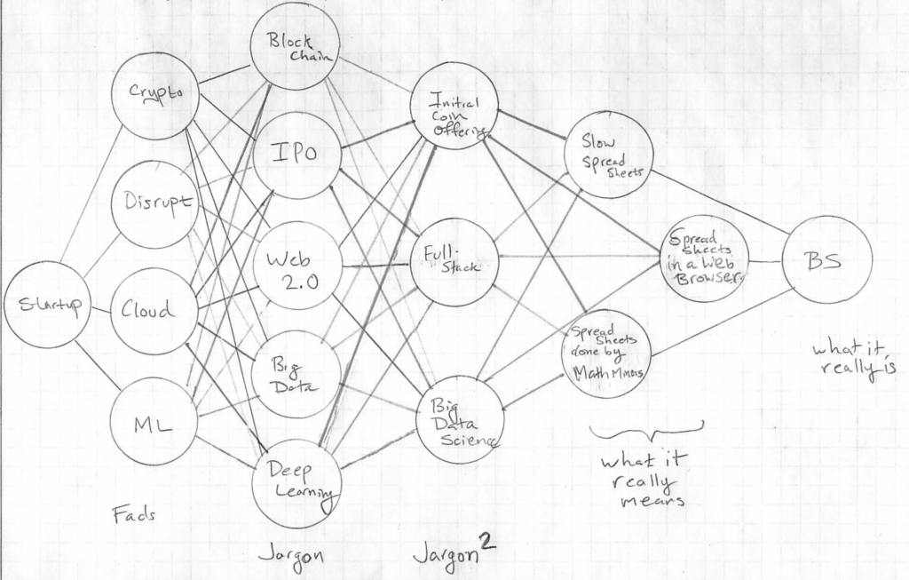
Although many neural networks have a ton of arcane connections and “hidden layers” (hidden only in that displaying them all is tedious), I have hand-drawn an example. This is a fully working neural network. My inspiration comes from participating in YCombinator’s Startup School over this summer. It solves the problem many of us keep running into: how to rapidly tell if a startup is BS (a bad startup).

This is a functional neural network. It takes in a set of words and decides if a start-up venture is a “bad startup” or not. It does not say whether the start-up is good; just is if it is a “bad startup.” At each layer, a series of keywords are in circles; if a sufficient number of these nodes get activated, then the neural network tells you that the idea is BS.

So, for example, if a startup is going to disrupt the cloud using crypto, and has a web 2.0 big data blockchain, you can assume their initial coin-offering, despite being full-stack, is really just a slow spreadsheet done in a browser by math minors. That’s BS man!

Many thanks to William Gasarch at UMD for inspiring this.

At Hacktech 2019, I intend to build a functioning prototype of the Guardia-NN system.

The hardware prototype system consists of the following:

A hardware device that features a huge button (representing “I DON’T WANT TO SEE THIS”) and an indicator (representing “YOU SAID YOU DON’T LIKE STUFF LIKE THIS”).

The device solves two problems at once: Firstly, people don’t like to see things that offend/traumatize them. But secondly, people generally don’t like being told by others (who may not share the same views and values) what is and is not offensive or triggering.

In other words, the machine serves as a guardian, using neural networks (hence the name Guardia-NN) — and replaces the almost universally reviled trope of the overly politically-correct “social justice warrior” with a machine. Now that’s automation we can all get behind!

It performs this task by picking up on user-defined trigger warnings (text tags that indicate that content will cause distress, offend, or otherwise bother the user), and relies on neural networks (large chains of decision making procedures) in order to learn from from repeated use what the end-user does and does not want to see. The device warns users that content ahead may trigger them, and allows them to navigate around said content with minimal exposure.

Because of its limited computational power, and reliance upon user interaction, it does not represent a feasible means of censoring others’ internet use. Rather, its intended use is to allow people to have a warning sign before exposure to content that may cause psychological harm and thus mitigate their exposure, akin to an allergen warning system.